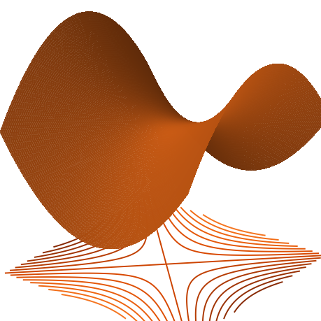
Graphs: Short interactive exercises from class, each in three levels: match functions of two variables to their graphs (which you can rotate) and to their contour diagrams. Every page checks your answers and can show the full answer key.

Introduction to Mathematica: Mathematica is a computational software suite we will use throughout the course. In this introduction, you will learn how to make basic caclulus computations and visualize multivariable functions, as well as where to find additional resources. Image: Wolfram.

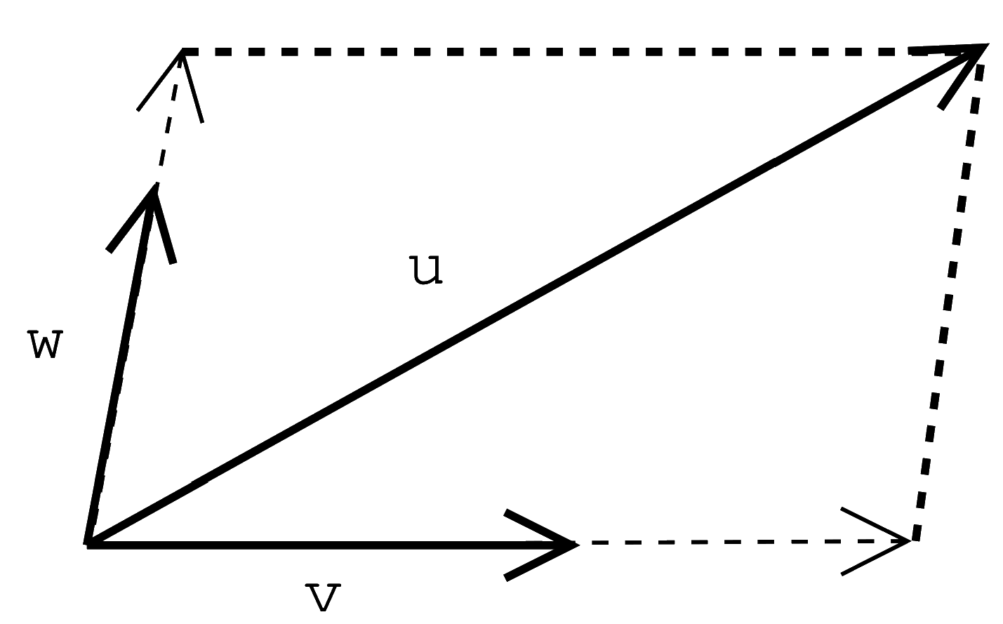
Lagrange multipliers in higher dimensions: In class, we discussed the method of Lagrange multipliers for functions of two variables subject to one constraint. What about functions with more variables and problems where there is more than one constraint?

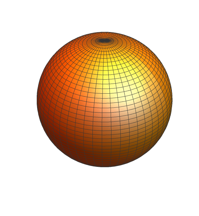
Volume of the sphere in n dimensions: The size of the set of points one unit from the origin depends on the dimension of the ambient space. This lab investigates how this quantity changes as the dimension increases. The results are not only important; they will surprise you!

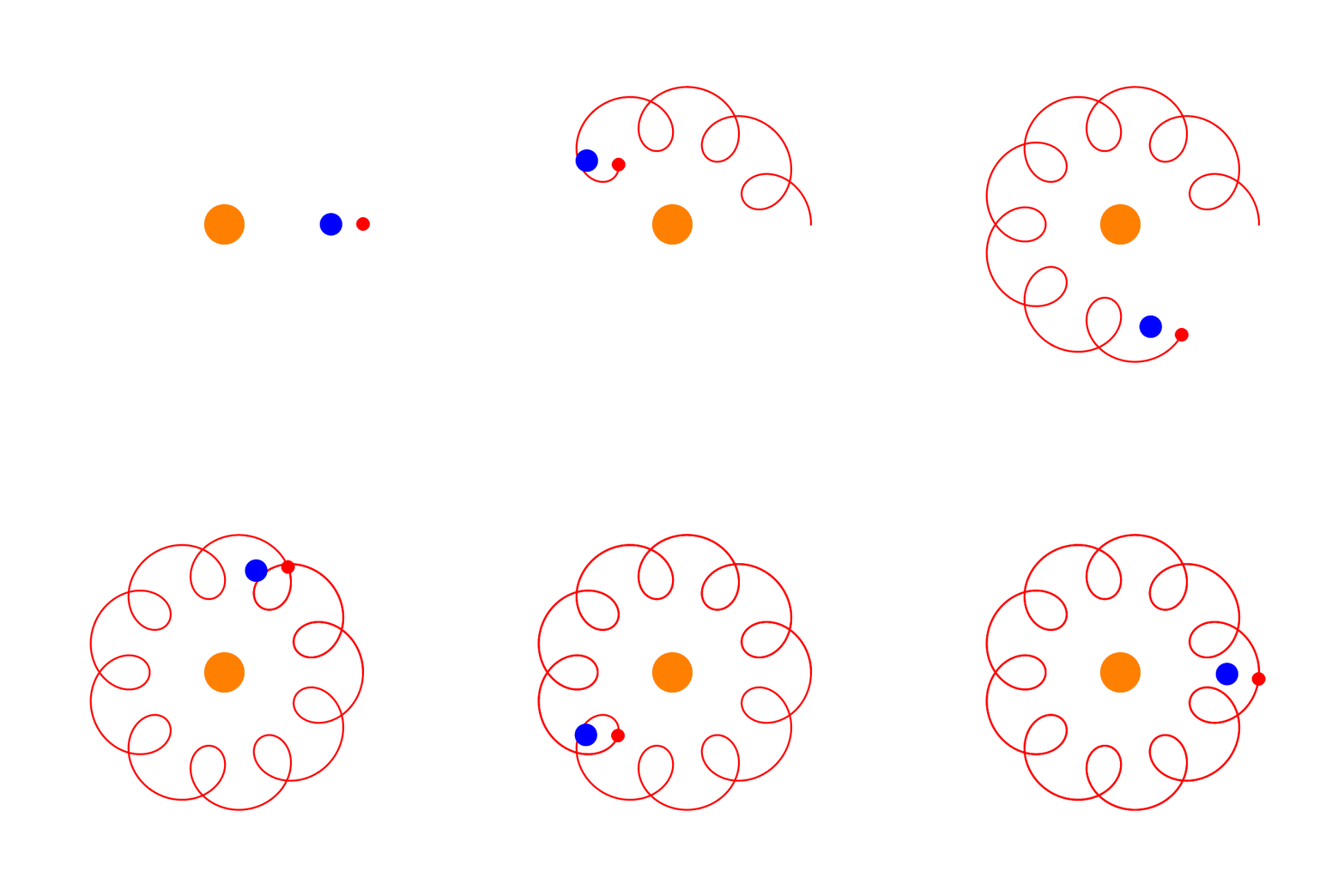
Parametric curves and celestial orbits: We will use parametric curves to study the orbits of celestial bodies in our solar system. As a result, we will settle an internet argument in the best possible manner: using mathematics.

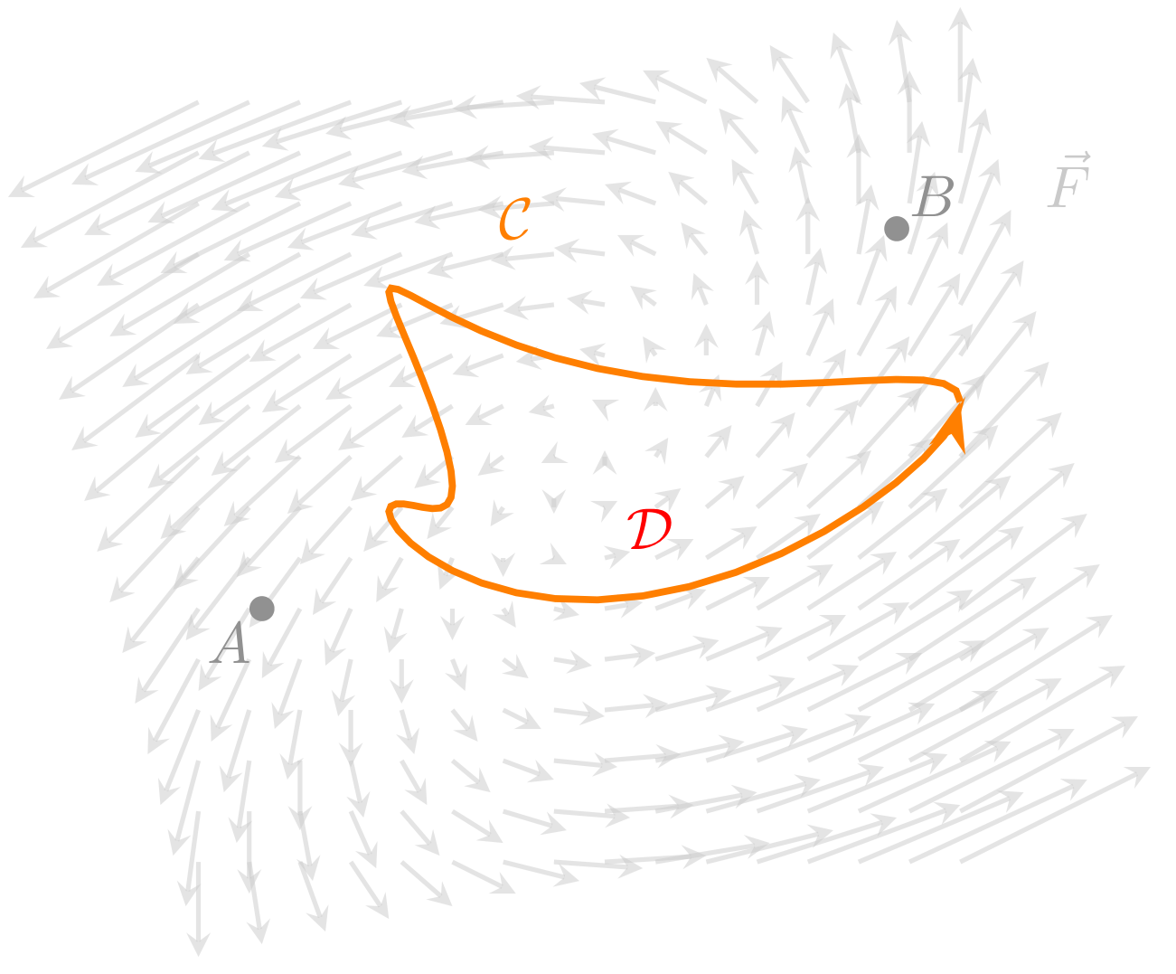
Path integrals: Some vector fields are nicer than others: they are often called path-independent or circulation-free and the calculations required to compute path integrals end up being simpler. We will experimentally figure out which ones these are and how one can tell.

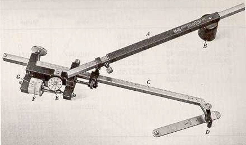
The planimeter: We analyze a nineteenth-century mechanical device that purports to measure area. The key idea comes from an novel use of Green’s Theorem about vector fields. Image: Laboratory Manual of Surveying